Physiographic Method
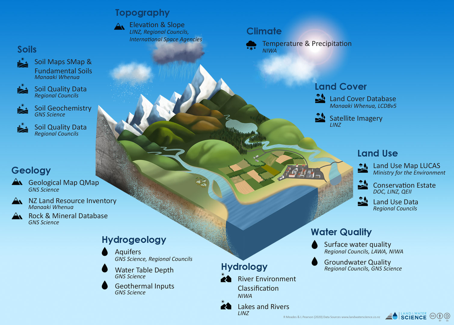
Researchers at Land and Water Science have developed a new methodology to integrate water quality data with existing map layers (such as soil, geology, topography, and land cover) to conceptualise and model the processes that control the spatial variability of water quality across New Zealand. Physiographic science works ‘backwards’, using the composition of water to trace the water’s journey back through the landscape to understand the landscape processes that control water composition and quality. Physiographics is based on the inherent (or natural) properties of the landscape.
The scientific approach was first developed in 2016 at Environment Southland and used by the council within its regional plan (Rissmann et al., 2016, Hughes et al., 2016). Since then, the method has evolved as part of the Our Land and Water National Science Challenge ‘Physiographic Environments of New Zealand’ project and was applied nationally with the support of several regional councils.
A Land and Water Science report is available through the following link that describes the Physiographic Environment Classification and the inherent susceptibility of the landscape for contaminant loss.
There are also three papers on the physiographic approach available through the following links:
How are Physiographic Environments mapped?
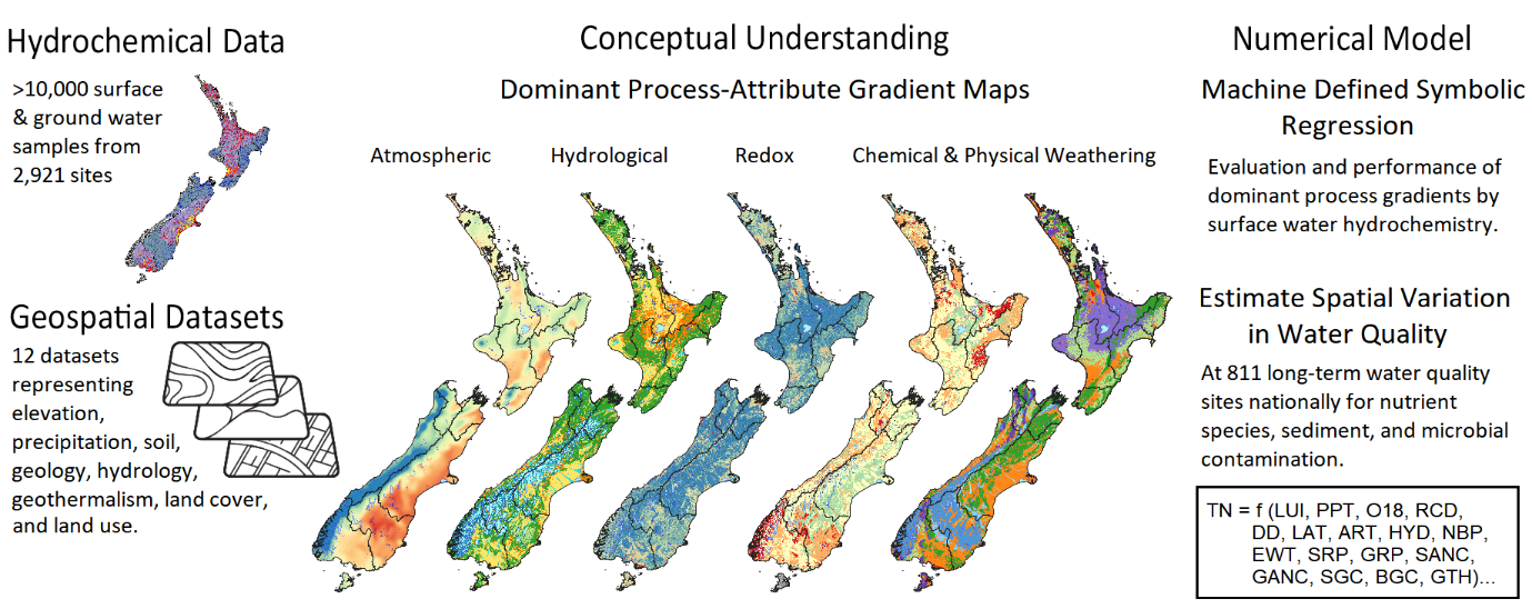
The physiographic method brings together map data for climate, topography, geology, soils, and hydrological controls with analytical chemistry at a national scale to produce a water quality specific landscape classification. The method utilised twelve pre-existing geospatial datasets (e.g., topography, soil, geology, land cover, climate, etc) and >10,000 ground and surface water samples from 2,921 monitoring sites across 8 regions of New Zealand.
A total of 16 process attribute gradient maps were defined nationally (2x climatic, 8x hydrological, 2x redox, 4x weathering, and 1x geothermal). Of these 16 maps the majority were classed according to hydrochemical measurement data from surface and groundwater sampled between 2014 and 2018. The process attribute gradient maps directly related to water quality (shaded) are available in Maps.
| Process | Process attribute gradient | PAG | Relevant datasets and scales | Attributes |
|---|---|---|---|---|
| Atmospheric | Precipitation (rain, snow, hail) source | O18 | 8 m DEM, δ18O-H2O precipitation isoscape (4 km2 pixel) | δ18O-H2O, altitude, distance from the coast |
| Precipitation volume | PPT | Annual average rainfall in mm (5 km2 pixel) | Precipitation volume | |
| Hydrological | Recharge domain and connectivity | RCD | Soil surveys (1:50,000), Aquifer type and extent (1:50,000) | Altitude, temperature isotherm, river network, Typic Fluvial Recent soils |
| Overland flow | OLF | Soil surveys (1:50,000), 8 m DEM | Soil texture, drainage class, permeability, slope, area of developed land | |
| Deep drainage (vertical drainage) | DD | Soil surveys (1:50,000) | Drainage class, permeability, depth to slowly permeable horizon | |
| Lateral drainage | LAT | Soil surveys (1:50,000) | Drainage class, permeability, depth to slowly permeable horizon, | |
| Artificial drainage | ART | Soil surveys, 8 m DEM, Land Cover (1 ha) | Drainage class, permeability, depth to slowly permeable horizon, slope, agricultural land cover | |
| Soil slaking and dispersion as a soil hydrological index | HYD | Soil surveys (1:50,000) | Soil texture, drainage class, permeability, area of developed land | |
| Natural soil zone bypass (cracking soil) | NBP | Soil surveys (1:50,000) | Cation exchange capacity, pH | |
| Equilibrium water table and aquifer potential | EWT | Water Table Model (0.04 km2 pixel) | Modelled water table depth | |
| Redox | Soil reduction potential | SRP | Soil surveys (1:50,000); soil chemistry profile points. | Drainage class, carbon content |
| Geological aquifer reduction potential | GRP | Geological surveys (1:50,000 - 1:250,000) | Rock type (main and sub rocks, geological descriptions) | |
| Weathering | Soil acid neutralization capacity | SANC | Soil surveys (1:50,000); geochemical baseline survey (8 km2) | Soil pH, cation exchange capacity |
| Geological acid neutralization capacity | GANC | Geological surveys (1:50,000 - 1:250,000); geochemical baseline survey (8 km2) | Rock type | |
| Surface/top regolith strength | SGC | Geological surveys (1:50,000 - 1:250,000) | Rock type and strength | |
| Basal regolith strength | BGC | Geological surveys (1:50,000 - 1:250,000) | Rock type and strength | |
| Geothermal | High enthalpy geothermal (≥180 °C) | GTH | Log of resistivity (limited to extent of Taupo Volcanic Zone) | Resistivity |
PAG: process attribute-gradient; DEM: digital elevation model
The process-attribute gradient (PAG) maps listed above were subsequently combined into Physiographic Environments guided by the performance to represent dominant processes controlling water quality. This involved ranking the process maps according to their sensitivity to generate landscape units. Where each unit, “Physiographic Environment,” is assumed to respond to land use pressure in a predictable and broadly similar manner.
The Physiographic Environments of New Zealand classification is hierarchical, with a basic 10 Environment Family Classification, and a higher-resolution Sibling Classification, which provides more information over water source and hydrological response (flow pathway), and the role the landscape has in removing or reducing potential water quality contaminants.
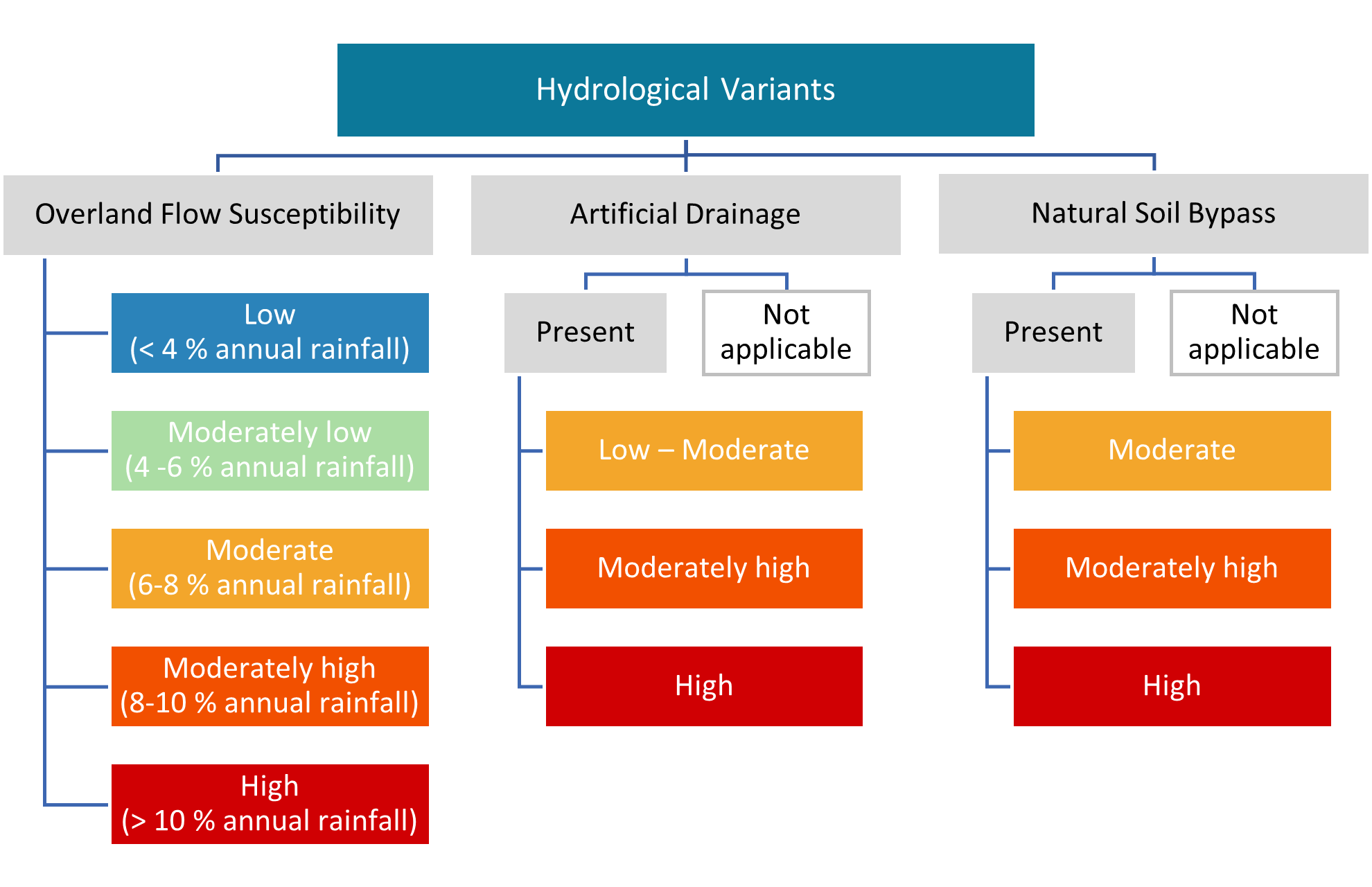
Associated with each classification level are hydrological variants. Variants provide additional detail where there is modification of the natural hydrology by artificial drainage, or seasonal and episodic variation in the pathway water takes to leave the land. During heavy rainfall events overland flow may become the dominant pathway or under dry or drought conditions, natural soil zone bypass may occur due to cracking soils. Variants change the predicted contaminant profile for the Physiographic Environment.
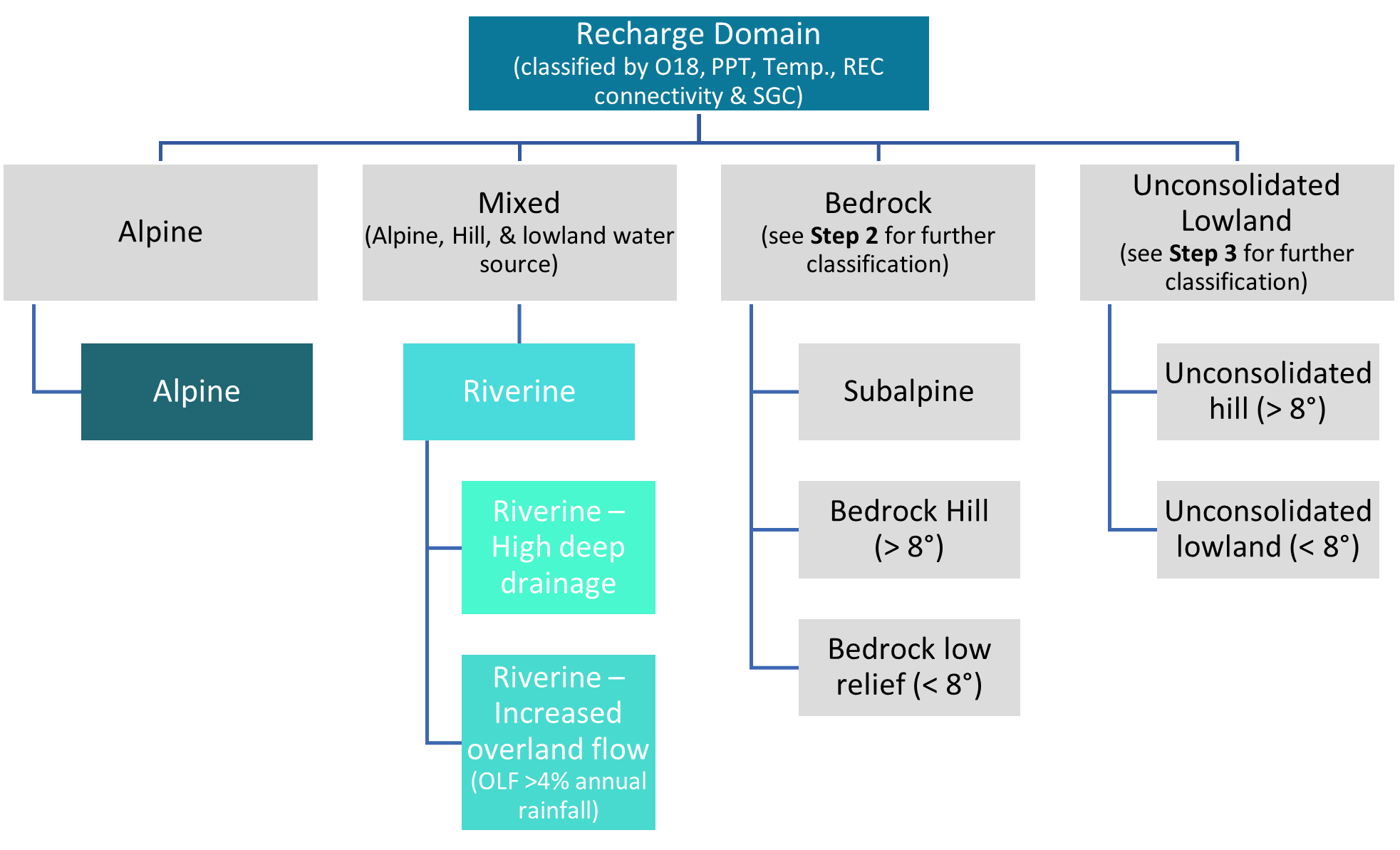
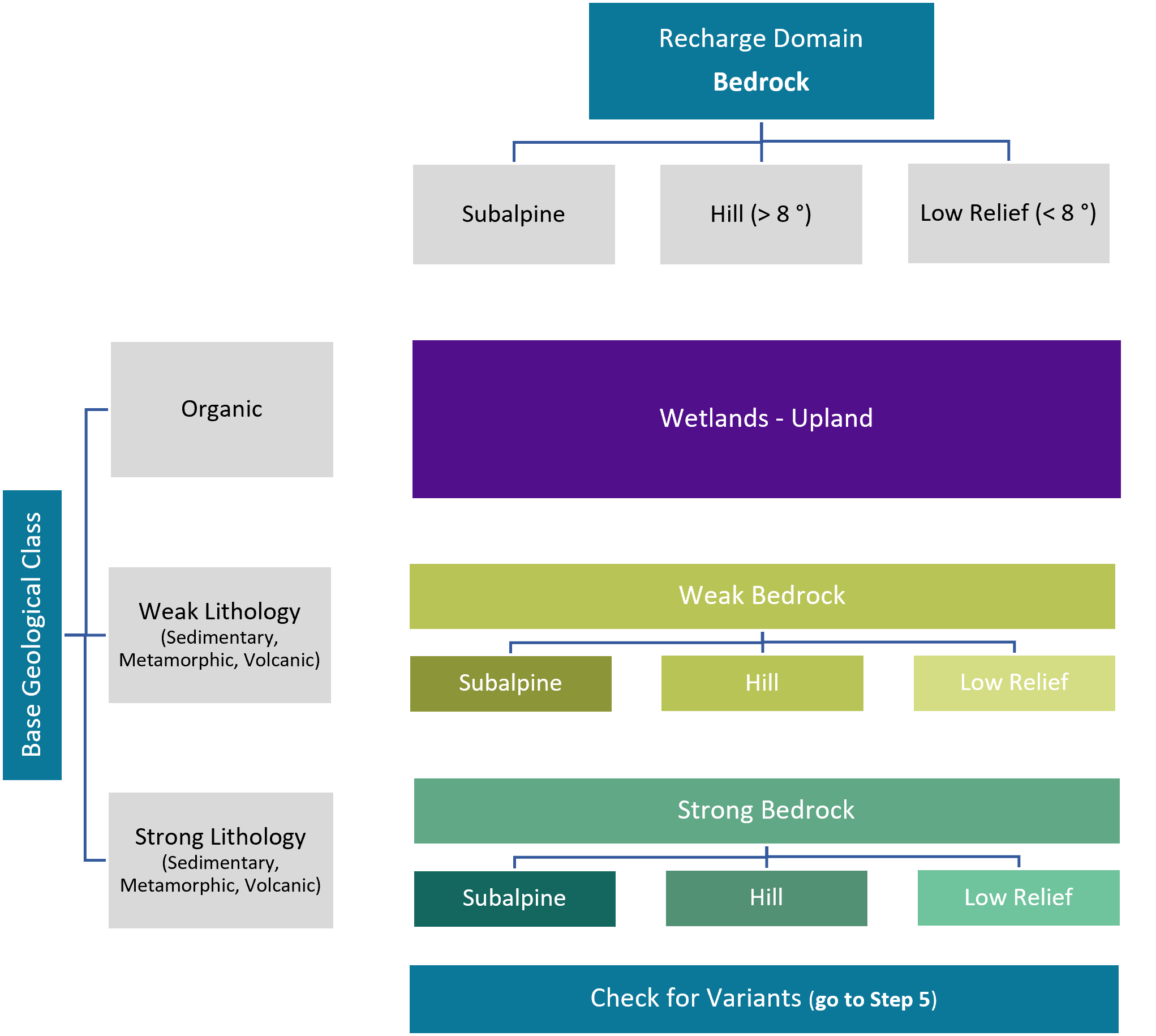
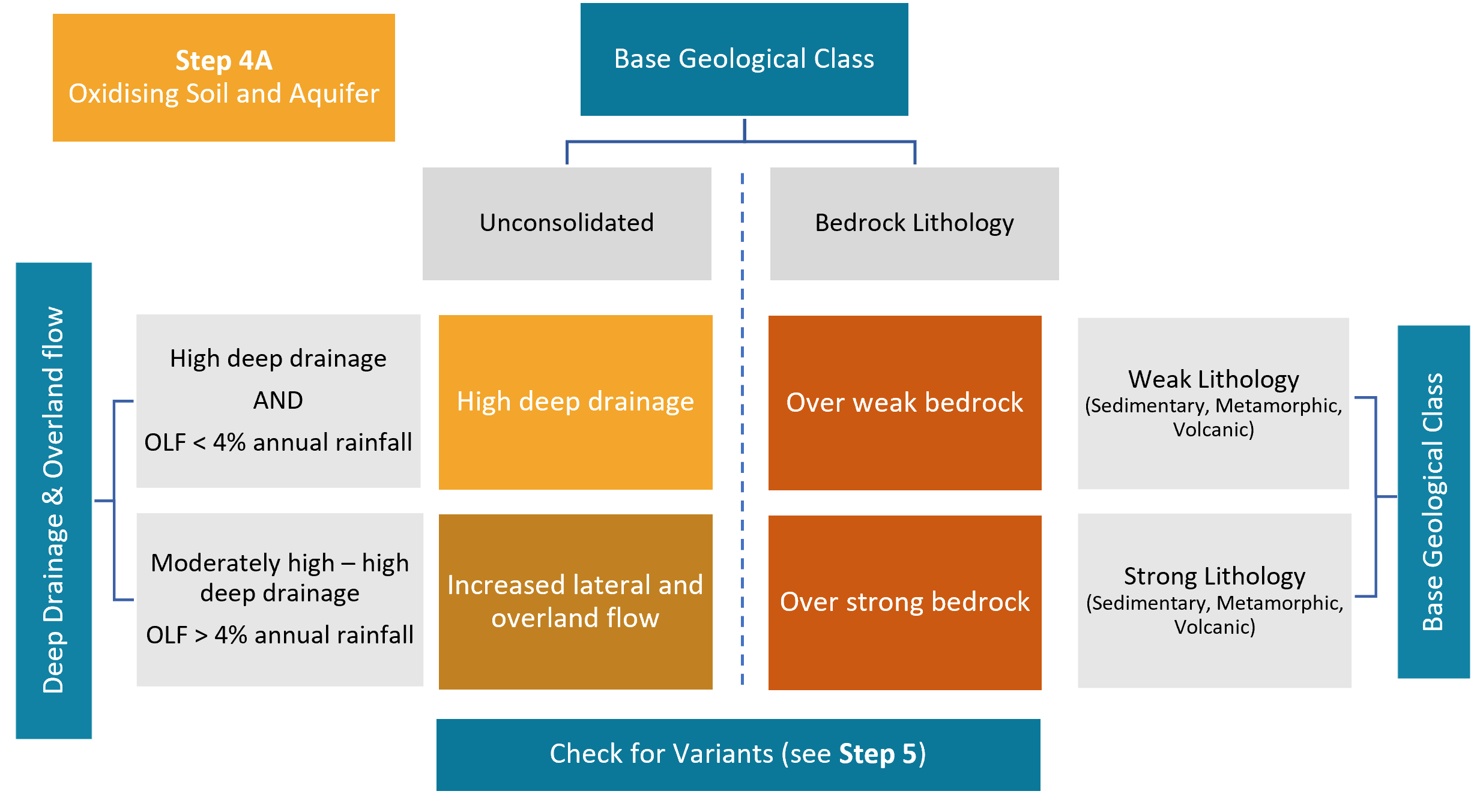
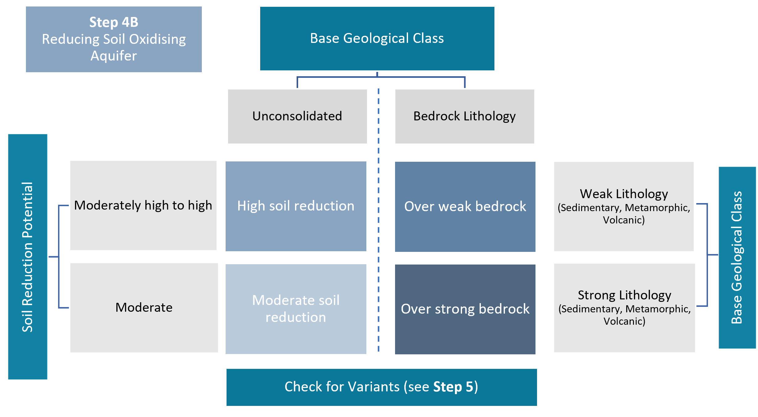
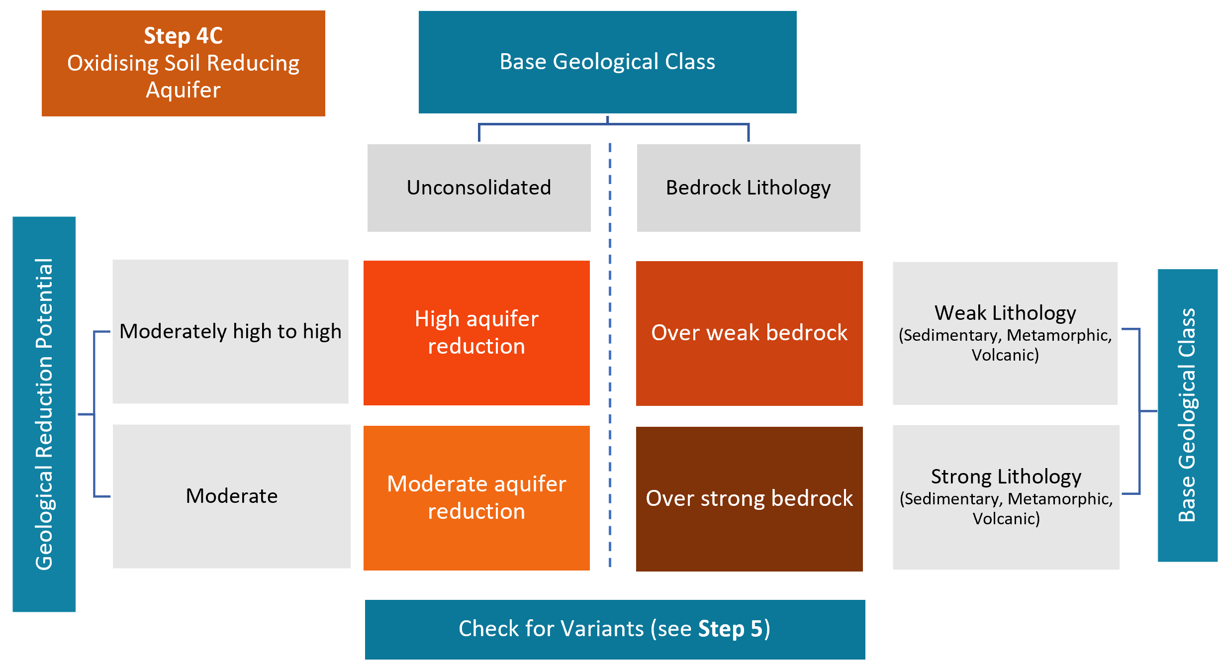
The following figures show the classification decision tree from Process-Attribute Gradient (PAG) to the Family and Sibling Classification (Step 1-4) and the identification of variants (Step 5). The classification of an environment is colour coded to match the map legends for the family and sibling classifications.
Step 1. Classification of macro scale hydrology (water source and connectivity) and Urban Environment.
Step 2. Classification of Upland Environments in Bedrock Recharge Domain.
Step 3. Classification of Unconsolidated Lowland Recharge Domain at Family Class.
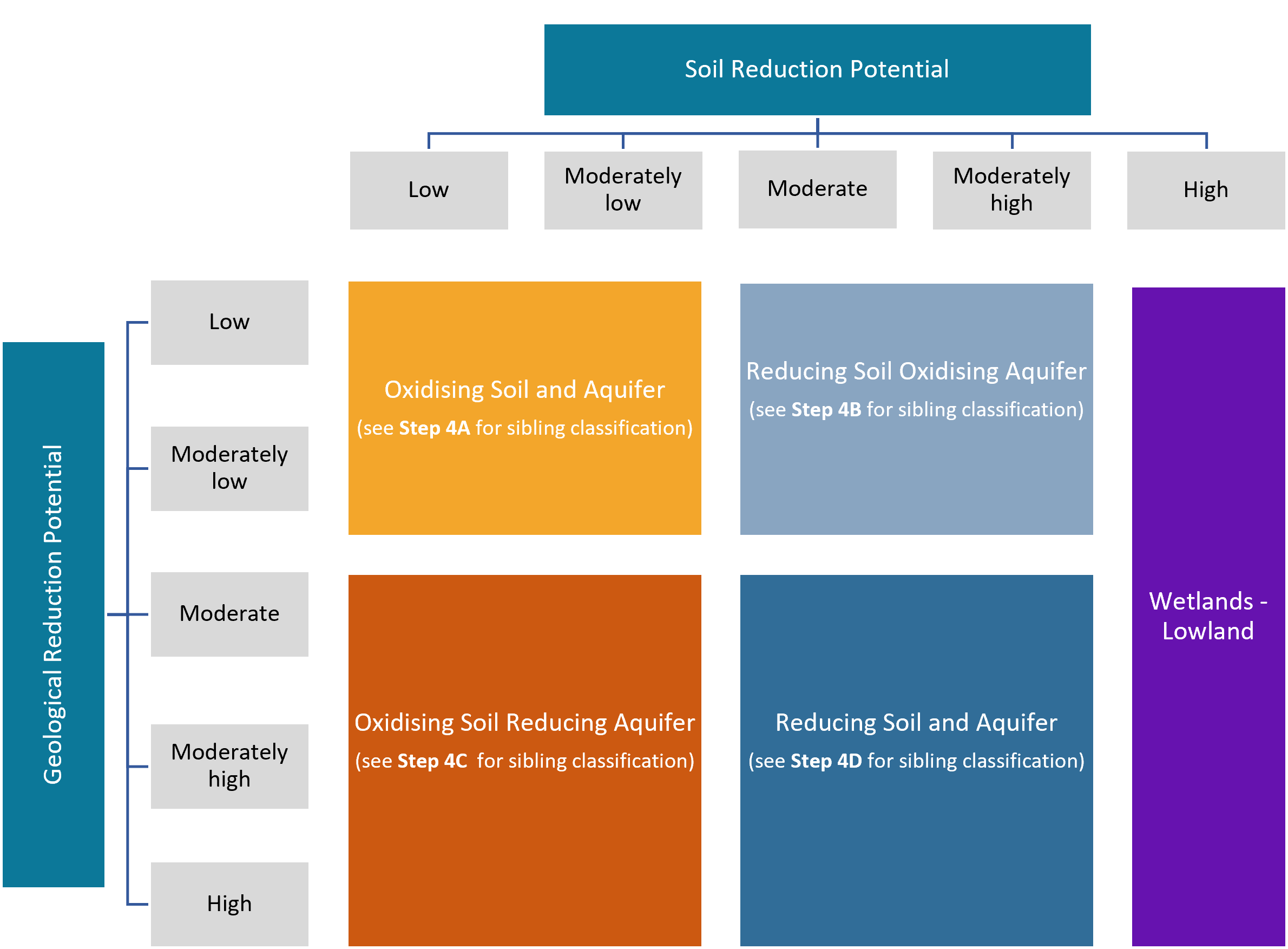
Step 4. Lowland Environments Sibling Classification.
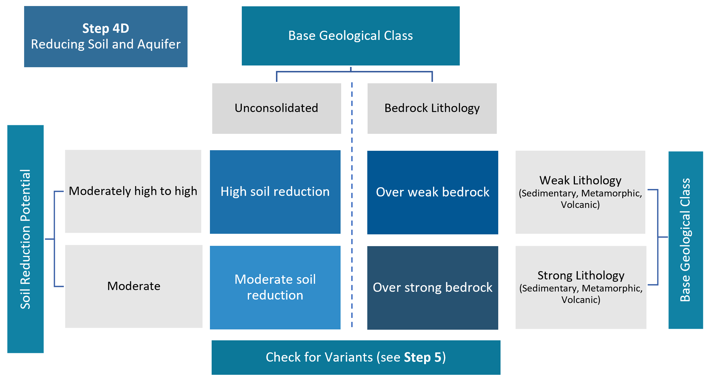
Step 5. Hydrological Variants apply in response to episodic rainfall events or seasonal variation and supersede the inherent risk of the Physiographic Environment when the pathway is active.
How is risk to water quality assigned?
Using the concepts of source (or supply) and transport limitation, the pattern(s) of contaminant generation can be predicted by the Physiographic Environment Classification. For example, a wider range of contaminants are likely to be generated from imperfectly to poorly drained agricultural soils during periods peak drainage. This reflects both adequate supply (e.g., land disturbance and contaminant source) and sufficient transport capacity (e.g., artificial drainage/overland flow). Conversely, contaminant generation from well-drained soils with high infiltration rates and equivalent land use pressure are likely to be lower under an equivalent land use pressure and precipitation intensity. In this case, the supply remains the same, but the transport capacity is reduced due to higher soil infiltration rates. In the first setting, the installation of artificial drainage is often used to mitigate the drainage limitation, effectively resulting in a similar outcome to the well-drained soil environment. However, mole-pipe drainage does not facilitate the same level of interaction between water and the soil matrix, and as a result, contaminants are often elevated in drainage discharges.
Collectively, these landscape factors interact to determine the differential sensitivity and magnitude of discharge of one or more contaminants to water. Therefore, water quality at a catchment-scale represents the outcome of multiple, spatially variable processes which influence the generation, transport, and transformation of contaminants across the contributing catchment.
Inherent landscape susceptibility for contaminant generation considers both the hydrological pathway contaminants take and how the landscape regulates water quality contaminants through dilution, resistance to erosion, filtration and adsorption, and attenuation of both N and P species. Each environment has distinct properties that can be used to predict the susceptibility of a contaminant for loss. The tables provided summarise for each Physiographic Family and Sibling class the hydrological pathway, the role of landscape in regulating contaminants, and the risk to the receiving environment defined as concentration and/or load to surface water, groundwater, or both. Where the landscape has a high regulating capacity it is good at reducing the risk to the receiving environment provided the specified hydrological pathway is active. When there is variation to the predicted hydrological response, variants apply. The variants may apply at different times of the year and modify the ability of the landscape to regulate contaminants. When active, the variant supersedes the predicted response for an environment.
The risk to water quality from agriculture, horticulture, forestry, and urban land uses (here after ‘land use’) for each Physiographic Environment is provided through a matrix by contaminant and species based on expert judgement and modelling. The risk matrix assumes a uniform source (land use pressure) in each environment for assigning risk, while the actual contribution from an area maybe significantly different depending on the actual land use type and intensity (i.e., native forest or high producing exotic grassland). This means for a high risk of loss to be realised, a contaminant source is required. This also applies to the variants where risk to water quality for all contaminants is significantly increased when bypass of the soil zone occurs by either overland flow, artificial drainage, or cracking soils. However, this risk is only realised if there is a contaminant source. For example, overland flow occurring in Alpine or natural state environments may be a relatively large volume of water, but the contaminant source load is low and the nutrient status of the sediment has not been enriched. These contributions to a receiving environment are generally considered background load.
Importantly, the risk assessment is preliminary and subject to refinement through an Our Land and Water, Sources to Sink project which aims to refine and improve the quantification of risk. This refinement will provide additional documentation and validation to support the landscape classification. In addition to this, an assessment of attenuation and uncertainty at various spatial scales will also be undertaken.
What is the scale of the classification?
The spatial scale of the information varies between the datasets used. The resulting map is generally at 1:50,000 which is accurate to approximately ±100m on the ground. Incorporating higher resolution datasets is the goal of future research.
What is the performance of the classification?
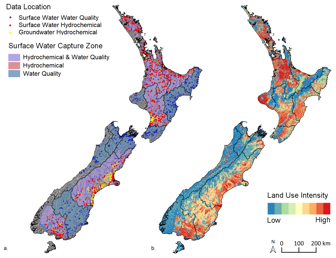
The ability of the process maps to represent steady-state water quality, as indicated by nitrogen and phosphorus species, sediment, and E.coli (a microbial indicator), was assessed by combining an independent dataset of 811 long-term surface water quality monitoring sites and a map representing the gradient in land-use intensity. The modelling identified regional climatic and geological variation as key controls on water quality variation across New Zealand.
The performance was tested using a statistical approach known as a coefficient of determination (R² value and pronounced “R squared”). An R² value of 1 indicates an exact match between the actual and predicted value or 100% accuracy and a 0 R² value indicates no relationship or 0% accuracy. As a rough rule of thumb, R² values of greater than 0.7 are considered strongly correlated, R² values between 0.5 and 0.7 are moderately correlated, R² values between 0.3 and 0.5 are weakly corelated, and an R² values less than 0.3 can be described as very weak or no correlation. A cross validated approach was also used. This means some of the measurement data used to test performance is withheld from the analysis during testing and swapped in and out to see how the R² value varies. A cross-validated R² value is considered more robust.
The process gradient maps were tested in regional subsets due to the significant variation in landscape processes and land use pressure. Cross validated R² values for environmental contaminants are listed below as a minimum-maximum and median performance:
- Total Nitrogen R² values ranged between 0.71 - 0.90 (median of 0.78)
- Nitrate-Nitrite Nitrogen R² values between 0.71 - 0.83 (median of 0.79)
- Total Phosphorus R² values between 0.63 - 0.85 (median of 0.73)
- Dissolved Reactive Phosphorus R² values between 0.57 - 0. 76 (median of 0.73)
- Turbidity between R² values 0.48 - 0. 92 (median of 0.69)
- Clarity between R² values 0.50 - 0. 89 (median of 0.62)
- E. coli between R² values 0.59 - 0. 75 (median of 0.74).
Learn more about these water quality indicators in SCIENCE – WATER QUALITY CONTAMINANTS.
Future work
Land and Water Science will be further developing this work through the Our Land and Water project ‘Mapping Contaminants from Source to Sink’ (S2S). The overall objective of the programme is to produce a national landscape classification for water quality to support contaminant risk assessment for policy option development. The classification units will describe contaminant processes within parcels of land, surface water, and shallow groundwater (hydrologically connected to streams and rivers). The classification, maps and supporting science will inform interchange between policy agencies, science and rural communities, iwi/hapū and industry.
The landscape classification will provide a system for identifying and grouping individual land parcels according to their risk for water quality, considering the substantial diversity of New Zealand’s landscapes. The S2S programme will define the inherent susceptibility of the landscape to contaminant yields matched to the vulnerability of receiving freshwater environments as part of a multi-contaminant framework that considers the risk response of varying land-use pressure in landscape classes. Improvement to PENZ can be made through the incorporation of additional inputs, such as the national groundwater redox map (Wilson et al., 2020), the internationally accepted RUSLE model for soil erosion that has recently been implemented using New Zealand spatial data (Donovan and Monaghan, 2021; Donovan, in press), and microbial pathogen risk. A key focus for this work will be the assessment of attenuation, uncertainties, and information gaps.